Polynomial equations are a fundamental element of algebra. Although they may seem daunting at first, mastering them is essential for a deeper comprehension of mathematical concepts. This guide covers three essential methods for solving polynomial equations: brute force, factoring, and synthetic division. By exploring these techniques, we aim to simplify the process of solving polynomial equations and provide valuable insights to improve your problem-solving skills.
Understanding polynomial eqn solving with bf fdg and sf
polynomial eqn solving with bf fdg and sf are mathematical expressions that involve variables raised to non-negative integer powers, each multiplied by a coefficient. These equations vary widely in complexity, from simple linear equations to intricate higher-degree polynomials. To tackle these equations effectively, it is essential to understand their fundamental structure.
Structure of polynomial eqn solving with bf fdg and sf
At the heart of a polynomial equation is a combination of terms linked by addition or subtraction. Each term consists of a coefficient (a numerical factor) and a variable raised to an exponent. For instance, the polynomial equation (2x^3 + 3x^2 – x + 5 = 0) is a third-degree polynomial. The degree of a polynomial is determined by its highest exponent, which indicates the polynomial’s complexity.
Classifying polynomial eqn solving with bf fdg and sf

Polynomial equations are categorized based on their degree, which helps in determining the appropriate solving method. Here are the common types:
- Linear Equations (Degree 1): These equations have the form (ax + b = 0) and represent a straight line when graphed.
- Quadratic Equations (Degree 2): Expressed as (ax^2 + bx + c = 0), these equations produce a parabolic curve.
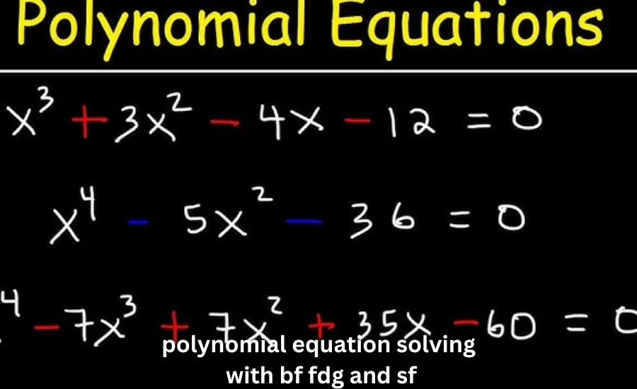
- Cubic Equations (Degree 3): With the form (ax^3 + bx^2 + cx + d = 0), cubic equations yield a cubic curve with potentially complex behavior.
- Quartic Equations (Degree 4): Represented as (ax^4 + bx^3 + cx^2 + dx + e = 0), quartic equations produce curves with more intricate patterns.
Understanding these categories allows you to choose the most effective method for solving each type of polynomial.
The Significance of polynomial eqn solving with bf fdg and sf
Polynomial equations are not just theoretical constructs; they have practical applications across various fields. They are used to model real-world phenomena such as:
- Physics: Describing the motion of objects and forces.
- Engineering: Analyzing structural designs and materials.
- Economics: Forecasting financial trends and economic growth.
- Computer Science: Algorithm development and data analysis.
Accurate solutions to polynomial eqn solving with bf fdg and sf are essential for making well-informed decisions in these and other domains.
The Brute Force Method
The brute force method is a straightforward approach to solving polynomial eqn solving with bf fdg and sf by testing multiple values to find the roots. While not the most efficient method, it provides a basic strategy for solving simpler equations or when other techniques are impractical.
Implementing Brute Force
- Identify a Range: Determine a reasonable interval within which potential solutions may lie. This involves estimating the possible values that could satisfy the polynomial equation.
- Test Values: Substitute different values from this range into the polynomial equation.
- Check for Zero: Identify which values make the polynomial equation equal to zero, thereby revealing the roots.
Advantages and Limitations
The brute force method is easy to understand and implement, making it ideal for beginners. However, it can be time-consuming and less practical for complex polynomials with multiple or intricate roots.
Example in Practice
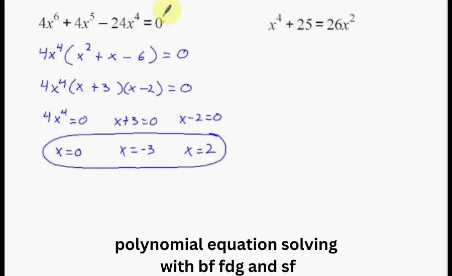
Consider the quadratic equation (x^2 – 5x + 6 = 0). By testing values within the range ([0, 3]), we discover that (x=2) and (x=3) are solutions, as they satisfy the equation by making it zero. This method is effective for simpler equations but becomes less feasible for more complex cases.
The Factoring Method
Factoring is a systematic approach that involves expressing a polynomial as a product of simpler polynomials. This method can streamline solving equations by breaking them into more manageable parts.
Understanding Factoring
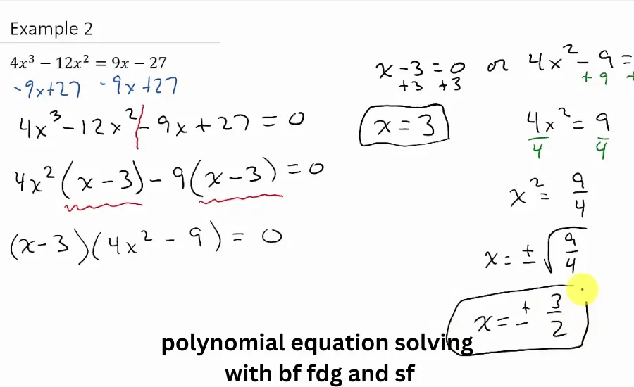
Factoring entails decomposing a polynomial into its fundamental factors. For instance, the quadratic polynomial (x^2 – 5x + 6 = 0) can be factored into ((x-2)(x-3) = 0), simplifying the solution process.
Techniques for Factoring
Several techniques are commonly used for factoring polynomials:
- Factoring by Grouping: This involves grouping terms in pairs and factoring out common factors from each group.
- Difference of Squares: Recognizes patterns such as (a^2 – b^2 = (a-b)(a+b)) to simplify equations.
- Factoring Trinomials: Breaks down trinomials into binomials, often using trial and error or the quadratic formula.
Example in Practice
For the quadratic equation (x^2 – 7x + 12 = 0), factoring yields ((x-3)(x-4) = 0). This factorization reveals that the solutions are (x=3) and (x=4), demonstrating how factoring can efficiently solve polynomial eqn solving with bf fdg and sf.
Synthetic Division
Synthetic division is a streamlined method for dividing polynomials, particularly useful for handling higher-degree polynomials. It simplifies the process by focusing on the coefficients and reducing the need for extensive calculations.
How Synthetic Division Works
Synthetic division involves dividing a polynomial by a linear factor using its coefficients, which simplifies the division process compared to traditional long division methods. It is particularly effective for dividing polynomials by linear factors.
Steps for Synthetic Division
- Set Up the Division: Write down the coefficients of the polynomial in descending order of their exponents.
- Perform the Division: Use the root of the divisor to carry out the division, applying a series of calculations to simplify the polynomial.
- Extract Results: Identify the quotient and any remainder from the division process.
Example in Practice
Consider dividing the polynomial (2x^3 + 3x^2 – 4x – 5) by (x – 1). Using synthetic division, we find the quotient to be (2x^2 + 5x + 1) and the remainder to be (-6). This demonstrates how synthetic division can efficiently handle polynomial division.
Mastering Polynomial Equations: Advanced Techniques and Practical Applications
polynomial eqn solving with bf fdg and sf are a cornerstone of algebra, essential for solving a wide range of mathematical problems. Although these equations can initially seem complex, mastering them is key to unlocking their full potential. This guide explores the advanced techniques for solving polynomial equations, focusing on how to effectively combine methods such as synthetic division, factoring, and brute force to achieve optimal results. By delving into these strategies, we aim to provide a comprehensive understanding of polynomial solving, enhancing both accuracy and efficiency.
Structure of Polynomial Equations
At their core,polynomial eqn solving with bf fdg and sf consist of multiple terms connected through addition or subtraction. Each term includes a coefficient (a numerical factor) and a variable raised to an exponent. For example, the polynomial equation (2x^3 + 3x^2 – x + 5 = 0) is a cubic polynomial, where the highest exponent (3) determines its degree. The degree of a polynomial indicates its complexity and dictates the most suitable methods for solving it.
Classifying Polynomial Equations
Polynomials are classified by the degree of their equations, and it is key to choose an appropriate method based on said type. The main categories include:
Linear Equations (Degree 1): Simplest type of polynomials represented as (ax + b = 0) They would graph with lines, as they have only one solution.
Quadratic Equations (Degree 2): Write it as: a(x^2) + b(x) c =0, If graphed will create parabola curves. They are factorable, can be solved through square roots or with the quadratic formula.
Cubic Equations (Degree 3): Polynomial equations of degree 3 with the form: (ax^3 + bx^2 + cx + d =0), cubic equation results in curves which are more intricate such as possible points inflection and multiple roots.
Quartic Equations (Degree 4): These represent quartic equations as (ax^4 + bx^3 + cx^2 + dx + e = 0), an example of a polynomial equation capable of producing complex curves with multiple turning points.
Being aware of these categories assists in determining which solution method is best suited to the degree and nature level each polynomial.
Practical Benefits of Combining Methods
In polynomial equation solving, integrating different techniques often leads to more effective results. By combining methods such as synthetic division and factoring, you can streamline the solution process and address complex equations more efficiently.
When to Combine Methods
Combining methods is particularly advantageous for higher-degree polynomials or equations with multiple variables. For instance, using synthetic division to simplify a polynomial before applying factoring can make the process more manageable. This approach allows for breaking down complex problems into simpler components, leading to clearer solutions.
Practical Example of Combined Methods
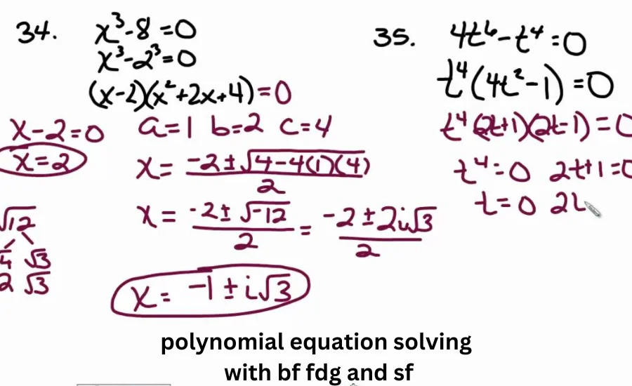
Consider the polynomial equation (x^3 – 6x^2 + 11x – 6 = 0). To solve this:
- Synthetic Division: Start by dividing the polynomial by (x – 1) using synthetic division. This step reduces the polynomial to (x^2 – 5x + 6).
- Factoring: Next, factor the resulting quadratic equation (x^2 – 5x + 6) into ((x – 2)(x – 3) = 0).
- Finding Roots: From this factorization, the roots of the original polynomial are (x = 1), (x = 2), and (x = 3). This combined approach efficiently reveals all the roots of the polynomial.
Advantages of a Combined Approach
Combining methods offers several distinct advantages:
- Enhanced Efficiency: Utilizing a combination of techniques can simplify complex equations, reducing the time and effort required to find solutions.
- Increased Accuracy: A systematic approach that integrates various methods helps avoid errors and ensures reliable results.
- Comprehensive Solutions: By leveraging the strengths of each method, you achieve a more thorough and effective solution strategy.
Real-World Applications of Polynomial Equations
Polynomial equations are not limited to theoretical mathematics; they have significant practical applications across various fields. Accurate solutions are crucial for addressing real-world challenges and driving progress in multiple industries.
Engineering and Physics: In engineering and physics, polynomial equations model and analyze complex systems, from structural integrity to dynamic motion. Accurate polynomial solutions are essential for designing safe structures, predicting material behavior, and optimizing performance in engineering applications. In physics, they help describe the motion of objects and the forces acting on them, contributing to the development of new technologies and innovations.
Economics and Finance: In the realms of economics and finance, polynomial equations are used to model and forecast economic trends and financial growth. They play a key role in analyzing market behaviors, making investment decisions, and planning economic strategies. Polynomial equations provide insights into patterns of economic activity and help in devising effective financial policies and strategies.
Computer Science: Polynomial equations are integral to various aspects of computer science, including algorithms, cryptography, and data analysis. They form the basis for many computational techniques, influencing software development, security protocols, and data processing methods. Understanding these equations is essential for advancing computational technologies and solving complex problems in the digital realm.
Common Challenges in Solving Polynomial Equations
Despite their importance, solving polynomial equations can present several challenges. Recognizing and addressing these challenges is essential for successful problem-solving.
Identifying Roots: Determining the roots of higher-degree polynomials can be particularly challenging due to their complexity. Employing accurate methods and reliable tools is crucial for obtaining correct solutions and avoiding potential errors.
Dealing with Complex Numbers: Polynomial equations with complex roots add another layer of difficulty. A thorough understanding of complex numbers and their properties is necessary for solving these equations effectively. Mastering complex number operations and their applications is vital for addressing such challenges.
Ensuring Precision: Precision is critical when solving polynomial equations, especially in applied contexts. Even minor inaccuracies can lead to significant consequences, highlighting the importance of meticulous calculations and validation.
Tools and Resources for Solving Polynomial Equations
Several tools and resources can enhance the process of solving polynomial equations, improving both efficiency and accuracy.
Online Calculators: Online calculators offer a convenient and user-friendly way to solve polynomial equations. They provide quick solutions and are particularly useful for performing rapid checks and validating results.
Software Programs: Advanced software programs, such as MATLAB and Mathematica, provide powerful capabilities for solving complex polynomial equations. These tools are invaluable for research, professional applications, and in-depth analysis, offering extensive functionality and precision.
Educational Resources: Educational resources, including textbooks, online courses, and tutorials, offer valuable knowledge and practice opportunities for mastering polynomial equations. These resources are essential for building a solid foundation, developing problem-solving skills, and gaining a deeper understanding of polynomial equations and their applications.
Final Words
polynomial eqn solving with bf fdg and sf are foundational to algebra and have broad applications across various fields. Mastering the methods of brute force (bf), factoring (fdg), and synthetic division (sf) equips you with essential tools for solving these equations. The brute force method provides a basic approach for simpler cases, while factoring offers a systematic way to simplify and solve polynomials. Synthetic division streamlines the process for higher-degree polynomials, enhancing efficiency. Combining these methods allows for a more comprehensive and effective problem-solving strategy. By understanding and applying these techniques, you can tackle polynomial eqn solving with bf fdg and sf with greater accuracy and confidence, benefiting both academic and practical applications.
For More relative Informaiton Visit TrendRevolve